Learning TensorFlow/Keras by polynomial regression
This is my attempt the learn artificial neural networks (ANNs) by breaking them down
into there constituent parts and running as simple code as possible.
Previously, I looked at linear regression
and how a neural network could be used to fit the data. This is an extension of that with more complicated data.
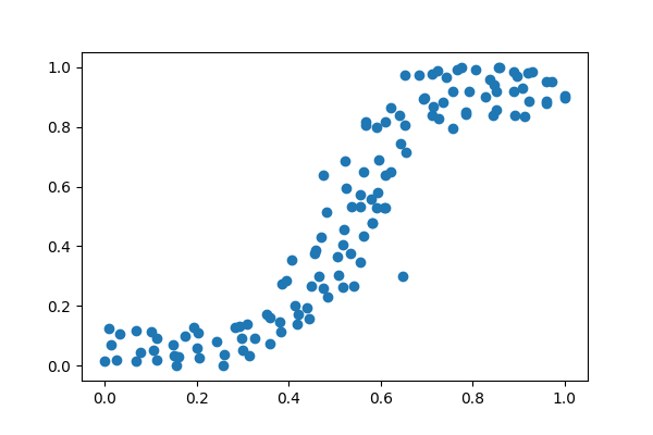
Firstly, I need to create some data. For this I used the DataCreator app, so that I could shape data.
Just as before I will fit the data using the tried and tested methods first. Here I will use Numpy's polyfit function to fit the data. From memory, I recognise this shape as a third order polynomial, meaning that it has the form ax3 + bx2 + cx + d. If I had forgotten this I would have simply brute-forced it and incremented the order in the polyfit function untill I could see that the model fit!
                p = np.poly1d(np.polyfit(X,y,3))
                t = np.linspace(0, 1, len(X))
                plt.plot(X, y, 'o', t, p(t), '-');
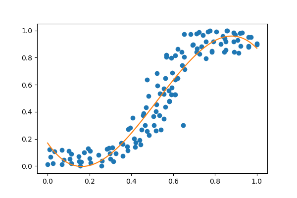
Looks good! We can see how many parameters were used to fit the model. As it is a third order polynomial we know that we need four parameters
poly1d([-5.23430684, 8.19136844, -2.25798128, 0.17015533])
Using the Pytorch website to make a manual attempt at fitting the parameters
                x =X
                # Randomly initialize weights
                a = np.random.randn()
                b = np.random.randn()
                c = np.random.randn()
                d = np.random.randn()

                learning_rate = 1e-5
                for t in range(1000000):
                    # Forward pass: compute predicted y
                    # y = a + b 2 + c x^2 + d x^3
                    y_pred = a + b * 2 + c * x ** 2 + d * x ** 3

                    # Compute and print loss
                    loss = np.square(y_pred - y).sum()
                    if t % 100 == 99:
                        continue
                        #print(t, loss)

                    # Backprop to compute gradients of a, b, c, d with respect to loss
                    grad_y_pred = 2.0 * (y_pred - y)
                    grad_a = grad_y_pred.sum()
                    grad_b = (grad_y_pred * x).sum()
                    grad_c = (grad_y_pred * x ** 2).sum()
                    grad_d = (grad_y_pred * x ** 3).sum()

                    # Update weights
                    a -= learning_rate * grad_a
                    b -= learning_rate * grad_b
                    c -= learning_rate * grad_c
                    d -= learning_rate * grad_d

                print(f'Result: y = {a} + {b} 2 + {c} x^2 + {d} x^3')
Now, for fun, we can try and let tensorflow learn what these parameters should be by trial and error.
                def build_model():
                    activation = 'linear'

                    input_layer = Input([1])
                    x_cubed = Lambda(lambda x:np.power(x,3))(input_layer)
                    x_squared = Lambda(lambda x:np.power(x,2))(input_layer)
                    hidden = Concatenate()([x_cubed,x_squared,input_layer])
                    output = Dense(1, activation = activation)(hidden)

                    model = Model(inputs=input_layer, outputs=output)

                    return model

                    def scheduler(epoch):
                        if epoch > 500:
                            return 0.1
                        elif epoch > 1000:
                            return 0.01
                        else:
                            return 0.5

                    callback = tf.keras.callbacks.LearningRateScheduler(scheduler)

                    optimizer = Adam()
                    model = build_model()
                    model.compile(loss='mean_squared_error',optimizer=optimizer)
                    history = model.fit(X,y,epochs=2000, verbose=2, callbacks=[callback])
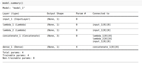
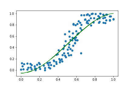
Here we are making use of the Lambda functions that allow us to make our own functions for use in the network. Because we know we need four parameters to fit the data the output from the network is a concatenation layer with four parameters in the form of a third order polynomial.

Success! The model was able to optimise the parameters and fit the data. Essentially all we have done is used Keras to make use of the Adam optimiser to fit our parameters. Obviously this was a much more inefficient solution to this problem than using the numpy poly1d function, but I am trying to learn the fundamentals of neural networks and machine learning and this exercise was a stepping stone.
The next step, for me, is to implement an optimisation algorithm on some basic data.
                #packages used
                import tensorflow as tf
                import numpy as np
                import matplotlib.pyplot as plt
                import keras
                from keras.models import Sequential, Model
                from keras.layers import Dense, Input
                from keras.optimizers import Adam
                from keras.layers import Lambda, Concatenate
                from scipy import stats
                from sklearn.preprocessing import MinMaxScaler