Learning TensorFlow/Keras by Linear regression

This is my attempt the learn artificial neural networks (ANNs) by breaking them down
into there constituent parts and running as simple code as possible.

Biological neurons

If my memory from my undergraduates days is correct, neurons are activated only once there is enough 'neurotransmitter' at the synapse. Then an electrical signal travels along the axon to whatever is at the other end - probably another neuron.

Artificial neurons (AN)

Were designed to replicate biological neurons. And so they essentially do the same thing, but with maths! If you need more than a laymans, half-remembered, explanation Google is your friend.

Learning how ANs work

First I need to make some data. I am going to create some data that makes sense to me and isn't just noise.

            
                def generate_data():
                    x = np.linspace(0, 1, 100)
                    y = 1.35 * x + np.random.randn(*x.shape) * 0.33 + 0.5
                    return x, y
                
                X, y = generate_data()

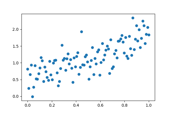
So, we can see we have some data that are positvely correlated.

Now I am going to make a model using TensorFlow and the Keras library.
If you don't understand Python perhaps this will not be for you.
All I am doing is creating a neural network with a single neuron

            
                def build_model():
                                
                    activation = 'linear'
                    
                    input_layer = Input(shape=[1])
                    output = Dense(1, activation = activation)(input_layer)
                    
                    model = Model(inputs=input_layer, outputs=output)

                    return model

My 'explanation' of the model and the basics of how it works

input_layer - literally the input (one dimensional vector) or 1 feature, no bias or weight. This is where we input the data that we think may help us predict whatever our target is - in this case the value of y. Output (Dense) - there is no 'output_layer' you use a dense layer which has a weight (w) and bias (b).

Weight = slope or gradient

Bias = intercept

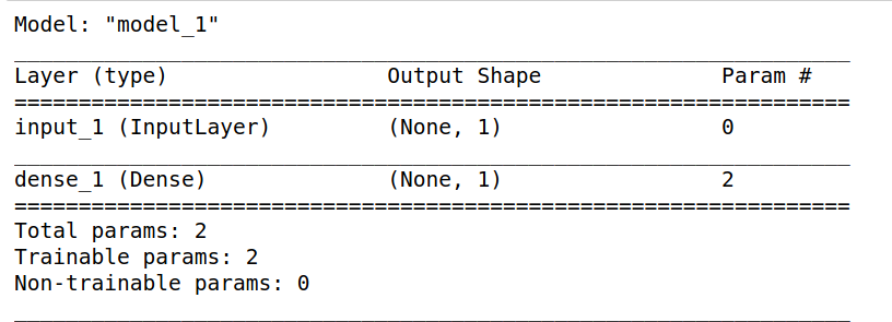
Essentially, weight and bias are both trainable parameters and we adjust them as needed. So this is why model.summary() gives a value of two. If we had a hidden dense layer in the middle with one unit how many trainable paramters would we have? Yep, 4.

As far as I am aware, this is the smallest possible functioning ANN that can fit 2 dimensional data. If we had a straigh horizontal line we could not use the bias paramter and only have a weight (use_bias = False)

Just like the equation of the line y = mx + c.
Each value passed into the neuron gets multiplied by w and b is added to the product - w(x) + b.
Hopefully the value the function returns is equal to y.

In this case I am using a linear activation function which just returns the input tensor - doesn't do anything.

As to how and when the activation is used, I believe if the value of w(x) + b exceeds a certain value (depends on the function) the the neuron is activated - gives output. Just like a biological neuron.

Weight = slope or gradient

Bias = intercept

Just like the equation of the line y = mx + c. Each value passed into the neuron gets multiplied by w and b is added to the product - w(x) + b. Hopefully the value the function returns is equal to y.

In this case I am using a linear activation function which just returns the input tensor - doesn't do anything.

Running the model

                
                optimizer = Adam(learning_rate = 0.6)
                model = build_model()
                model.compile(loss='mean_squared_error',optimizer=optimizer)
                history = model.fit(X,y,epochs=30, verbose=0)
                model.summary()

Now to check the performance

                
                    slope, intercept, r_value, p_value, std_err = stats.linregress(X,y)
                    plt.scatter(X,y)
                    plt.plot(X,model.predict(X), color = 'r', label = 'neural-net')
                    plt.plot(X, X*slope + intercept, color = 'g', label = 'lin-regress')
                    plt.legend()
                    plt.savefig('final-fig.png', dpi = 100)

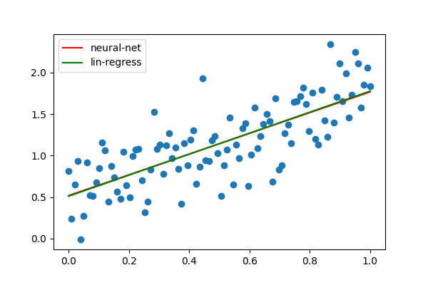
The artificial neuron fit almost perfectly!

                    
                    w, b = model.layers[1].get_weights()
                    m, c = slope, intercept

                    print(f'weight {w[0][0]:.2f}, gradient {m:.2f},\nbias {b[0]:.2f}, intercept {c:.2f}')

                    weight 1.25, gradient 1.27,
                    bias 0.52, intercept 0.51

So now the question is, how are the weights and biases updated?

My assumption: After each epoch, the weights and biases are adjusted, randomly-ish and if the accuracy improves it carries on adjusting in that direction, if it decreases it changes direction. How these values are changed depends on the optimizer in my case Adam?

The parameter learning_rate is how big the steps are in the changes the network makes to the weights and bisases, the default is 0.001. When I left it default with 1000 epochs the weight and bais was equal to the results of linear regression. I have seen people adjust this dynamically so the learning rate becomes slower over time - takes smaller steps to hone in on the true value.

I guess it is a trade-off between speed and accuracy - yet another parameter to optimse!

In the next post about this I shall try and fit some polynomial data, and hopefully learn how the weights and biases are changed